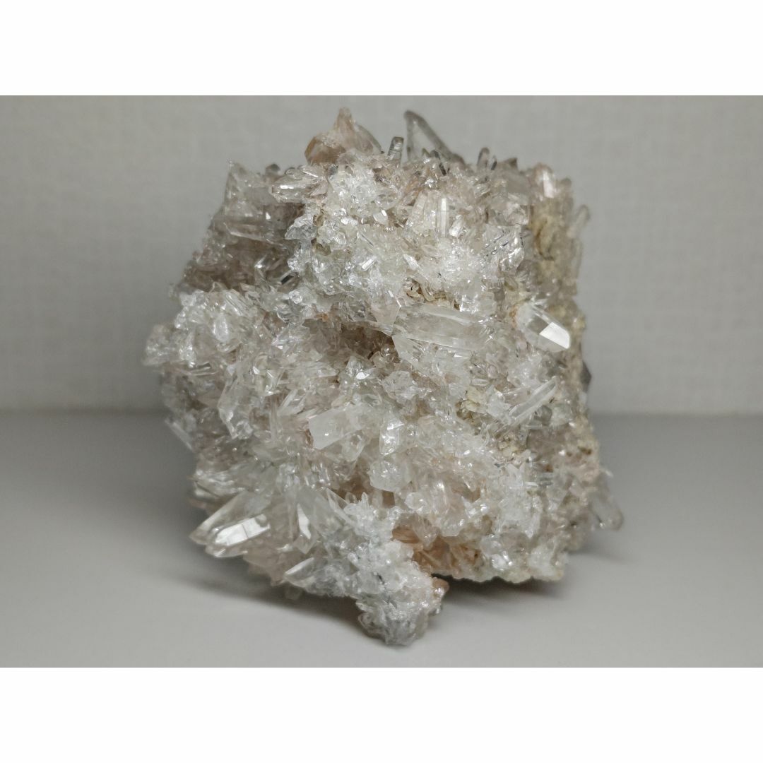
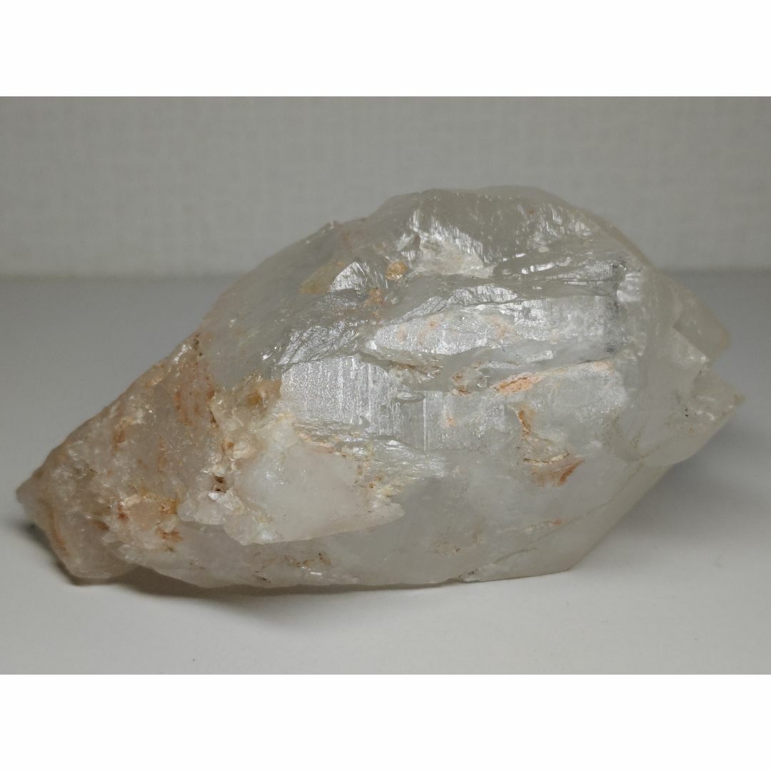
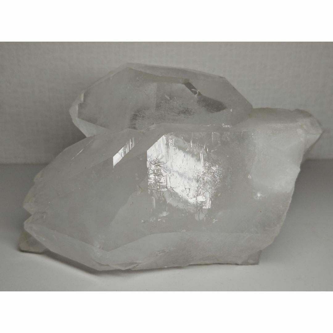
水晶 1.2kg クォーツ 原石 鑑賞石 自然石 誕生石 宝石 鉱物 鉱石 水石
(税込) 送料込み
商品の説明
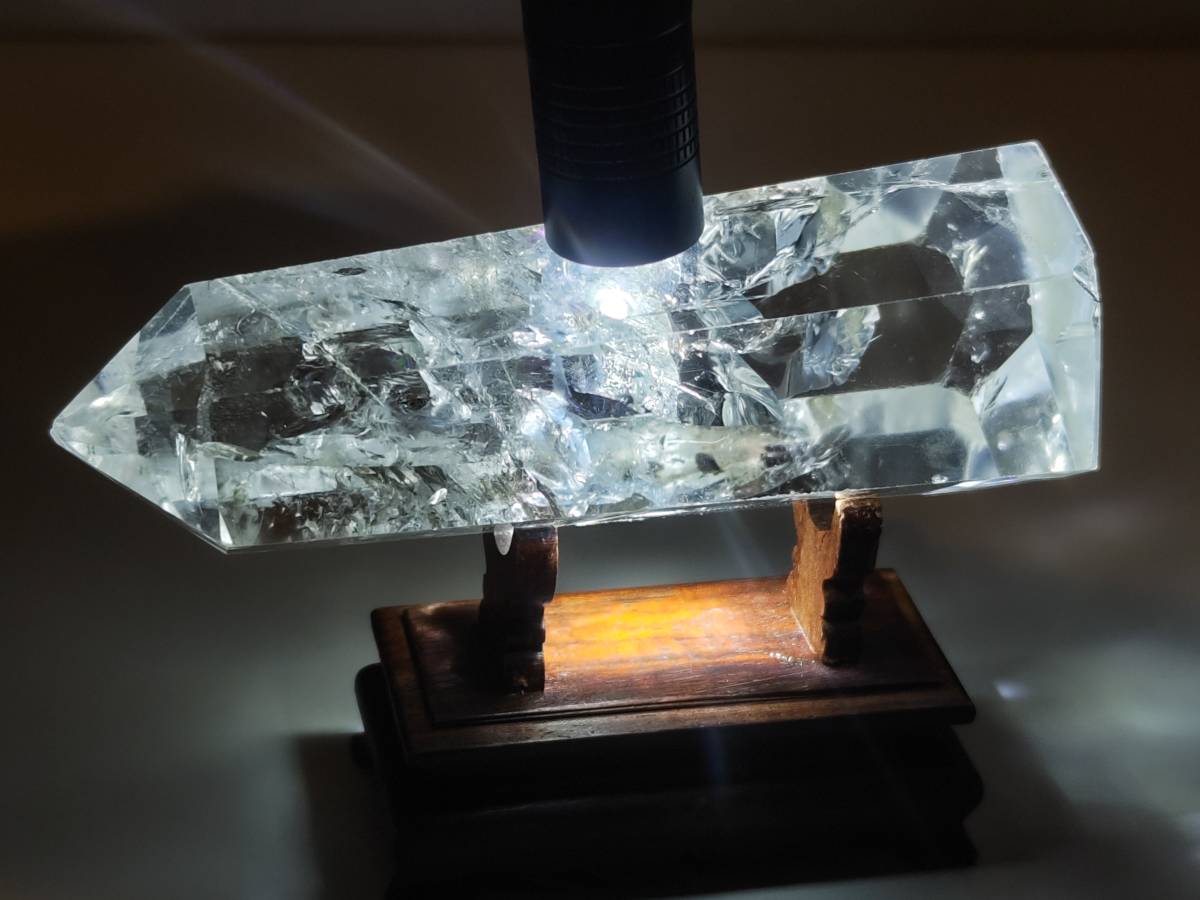
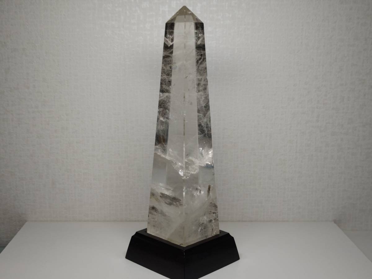
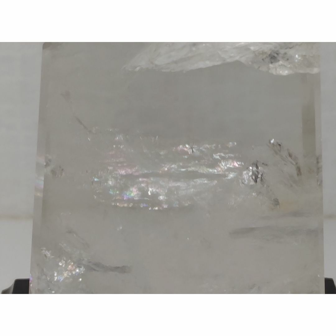
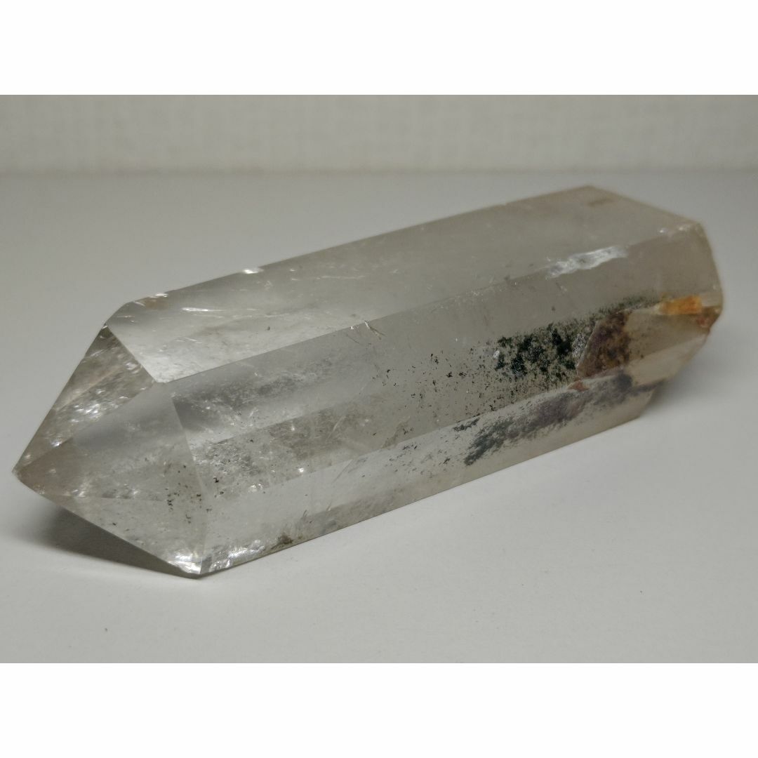
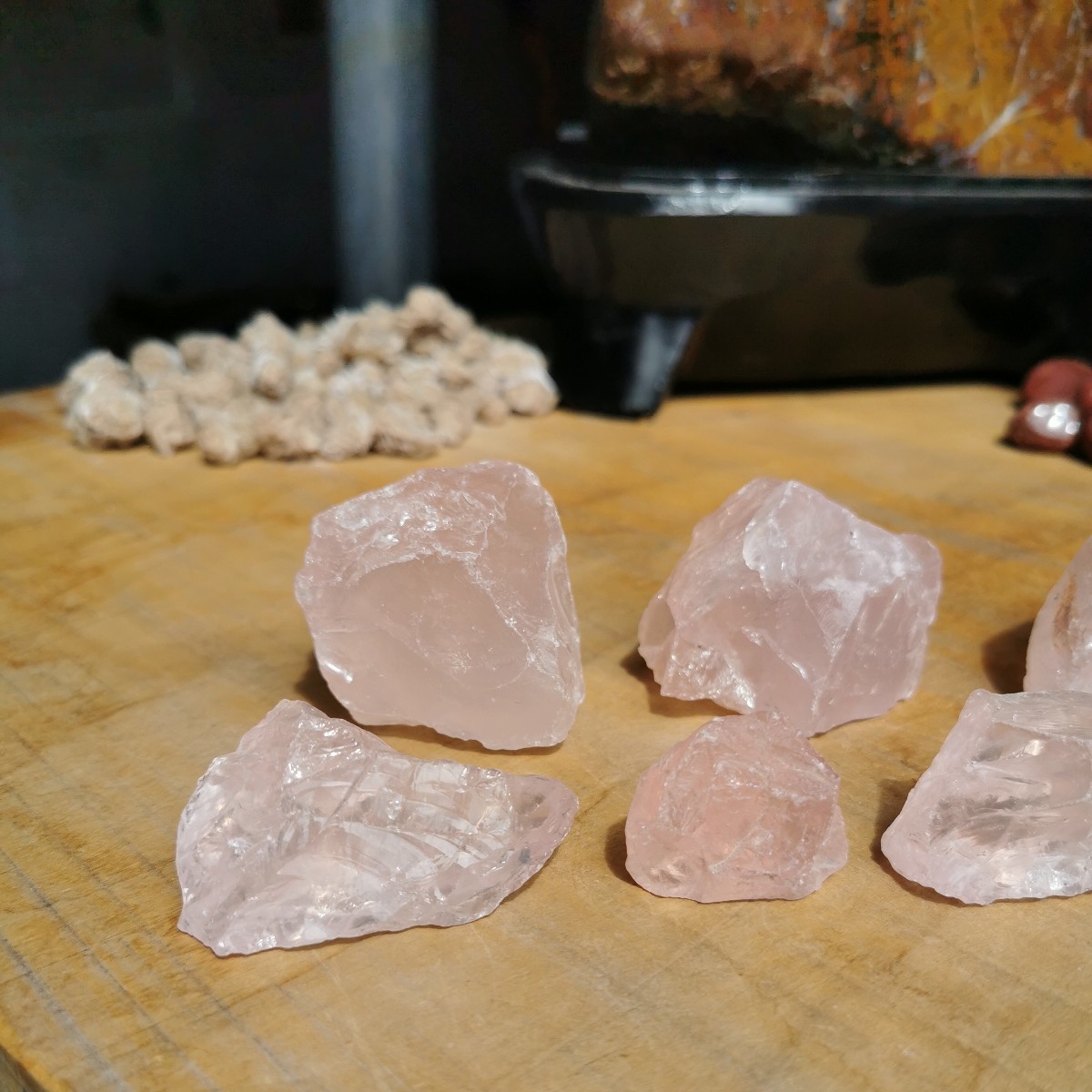
きれいな水晶オベリスクです。
【サイズ】約26cm×9cm×8.5cm
【重 量】1210g
注意事項
1.モニターによっては画像と実際の商品の色合いが異なって見える場合(商品によっては濡らした状態で撮影している場合もあります)がございます。また、ヒビ、キズ、研磨痕等細部までこだわる方、神経質な方は入札をご遠慮ください。
1.出品物について、一部の商品を除き鑑別・鑑定等は行ってはおりません。仕入(購入)元からの情報や自己判定により出品しており、本物保証するものではありません。また、鉱物のなかにはその特定が難しいものもあり、商品説明やタイトルに誤った記載がされる場合がある旨、ご承知ください。
1.商品の発送にあたっては、きちんと梱包して発送させていただきますが、配送にともなう万一の事故(紛失や破損等)については、各配送業者の補償での対応とさせていただきます。当方での補償はございませんので、ご注意くださいませ。
1.商品については他のサイトでも出品しております。ご購入のタイミングによっては、キャンセルとさせていただく場合がございますので、予めご承知下さいませ。商品の情報
| カテゴリー | おもちゃ・ホビー・グッズ > コレクション > その他 |
|---|---|
| 商品の状態 | 目立った傷や汚れなし |

水晶 1.2kg クォーツ 原石 鑑賞石 自然石 誕生石 宝石 鉱物 鉱石 水石-

水晶 1.2kg クォーツ 原石 鑑賞石 自然石 誕生石 宝石 鉱物 鉱石 水石

水晶 1.2kg クォーツ 原石 鑑賞石 自然石 誕生石 宝石 鉱物 鉱石 水石

水晶 1.2kg クォーツ 原石 鑑賞石 自然石 誕生石 宝石 鉱物 鉱石 水石
水晶 676g クォーツ 原石 鑑賞石 自然石 誕生石 宝石 鉱物 鉱石 水石

水晶 1.2kg クォーツ 原石 鑑賞石 自然石 誕生石 宝石 鉱物 鉱石 水石

水晶 889g クォーツ 原石 鑑賞石 自然石 誕生石 宝石 鉱物 鉱石 水石-
水晶 1.2kg クォーツ 原石 鑑賞石 自然石 誕生石 宝石 鉱物 鉱石 水石
水晶 1.2kg クォーツ 原石 鑑賞石 自然石 誕生石 宝石 鉱物 鉱石 水石

水晶 498g クォーツ 原石 鑑賞石 自然石 誕生石 宝石 鉱物 鉱石 水石-

水晶 1.2kg クォーツ 原石 鑑賞石 自然石 誕生石 宝石 鉱物 鉱石 水石-
水晶 803g クォーツ 原石 鑑賞石 自然石 誕生石 宝石 鉱物 鉱石 水石-

水晶 928g クォーツ 原石 鑑賞石 自然石 誕生石 宝石 鉱物 鉱石 水石-

水晶 676g クォーツ 原石 鑑賞石 自然石 誕生石 宝石 鉱物 鉱石 水石

水晶 549g クォーツ 原石 鑑賞石 自然石 誕生石 宝石 鉱物 鉱石 水石-
販売特注品 水晶 ・168g クォーツ 原石 鑑賞石 自然石 誕生石 鉱石

水晶 1.9kg クォーツ 原石 鑑賞石 自然石 誕生石 宝石 鉱物 鉱石 水石

水晶 676g クォーツ 原石 鑑賞石 自然石 誕生石 宝石 鉱物 鉱石 水石

ラピスラズリ 2.1kg 原石 鑑賞石 自然石 誕生石 水石 宝石 鉱物 鉱石-
水晶 ・1.2kg クォーツ 原石 鑑賞石 自然石 誕生石 鉱石 鉱物 水石

水晶 1.2kg クォーツ 原石 鑑賞石 自然石 誕生石 宝石 鉱物 鉱石 水石-
水晶 549g クォーツ 原石 鑑賞石 自然石 誕生石 宝石 鉱物 鉱石 水石-

水晶 2.8kg クォーツ 原石 鑑賞石 自然石 誕生石 宝石 鉱物 鉱石 水石-

ラピスラズリ 1.2kg 原石 鑑賞石 自然石 誕生石 水石 宝石 鉱物 鉱石-

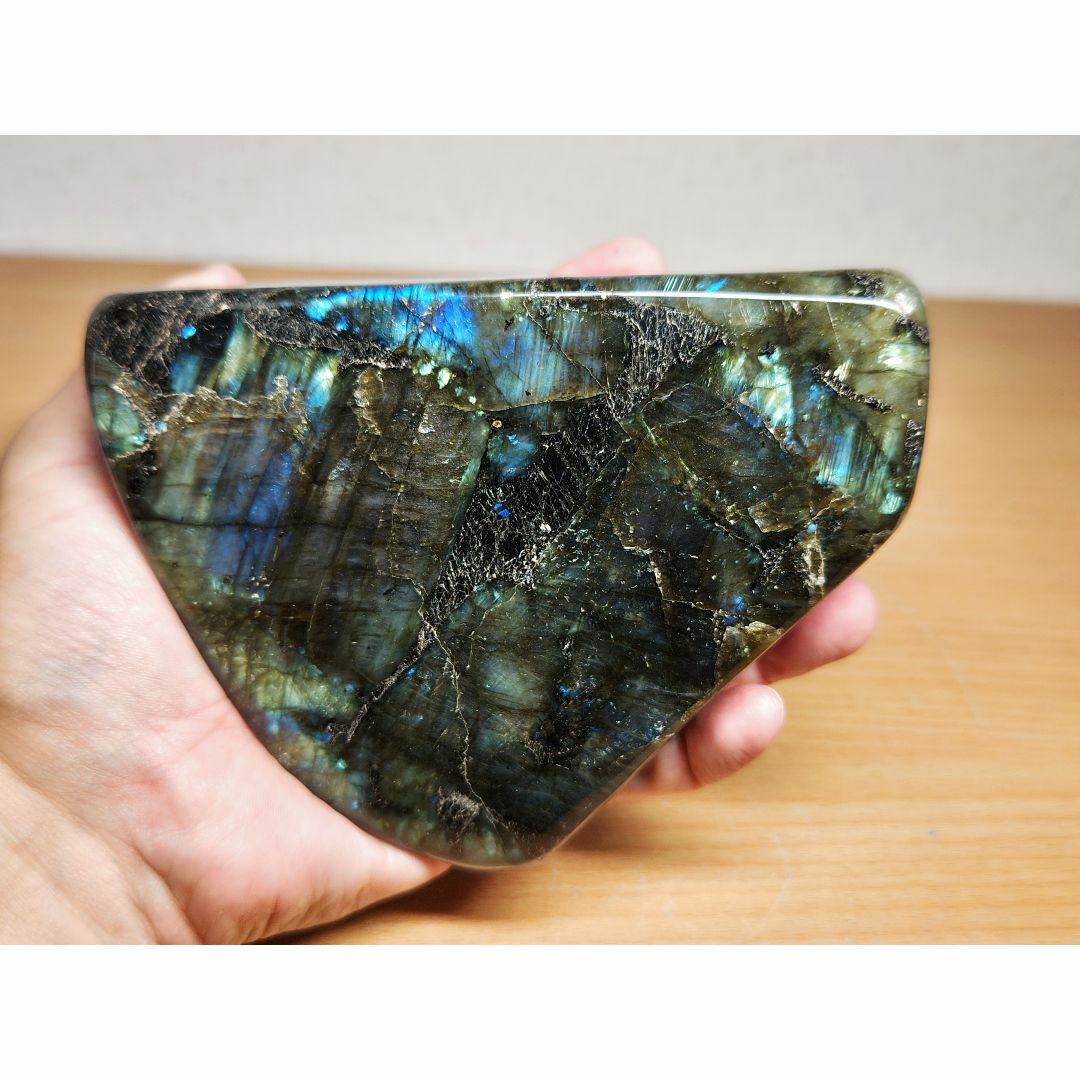
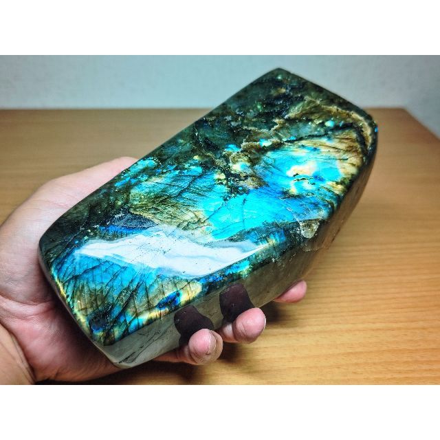
ラブラドライト 700g 鑑賞石 原石 自然石 鉱物 水石 誕生石 宝石 鉱石-
水晶 549g クォーツ 原石 鑑賞石 自然石 誕生石 宝石 鉱物 鉱石 水石-
水晶 1.9kg クォーツ 原石 鑑賞石 自然石 誕生石 宝石 鉱物 鉱石 水石
水晶 ・1.2kg クォーツ 原石 鑑賞石 自然石 誕生石 鉱石 鉱物 水石

水晶 1.2kg クォーツ 原石 鑑賞石 自然石 誕生石 宝石 鉱物 鉱石 水石-

水晶 549g クォーツ 原石 鑑賞石 自然石 誕生石 宝石 鉱物 鉱石 水石-
水晶 676g クォーツ 原石 鑑賞石 自然石 誕生石 宝石 鉱物 鉱石 水石
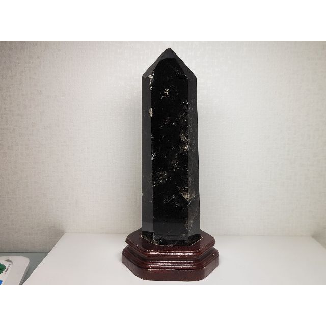
黒水晶 2.1kg 水晶 クォーツ オベリスク 原石 鑑賞石 自然石 誕生石
水晶 1.2kg クォーツ 原石 鑑賞石 自然石 誕生石 宝石 鉱物 鉱石 水石

ラブラドライト 700g 鑑賞石 原石 自然石 鉱物 水石 誕生石 宝石 鉱石-

ラピスラズリ 1.2kg 原石 鑑賞石 自然石 誕生石 水石 宝石 鉱物 鉱石-
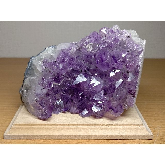
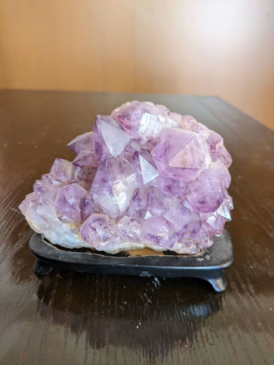
紫水晶 982g クォーツ アメジスト 原石 鑑賞石 自然石 誕生石 宝石 鉱物-
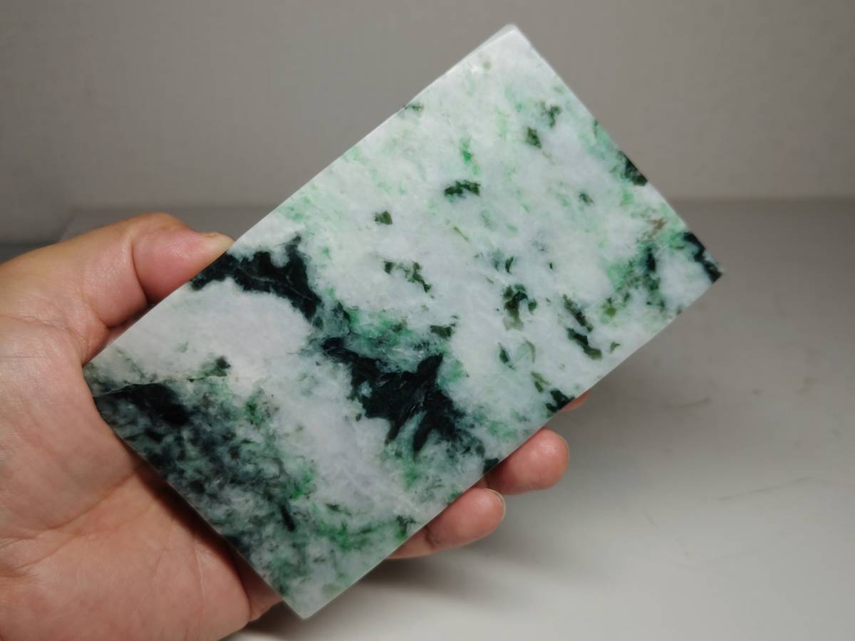
最短翌日着 【白緑】 ☆615g☆ 翡翠 原石 ヒスイ 鉱物 鑑賞石 糸魚川
水晶 549g クォーツ 原石 鑑賞石 自然石 誕生石 宝石 鉱物 鉱石 水石-
ラブラドライト 700g 鑑賞石 原石 自然石 鉱物 水石 誕生石 宝石 鉱石-
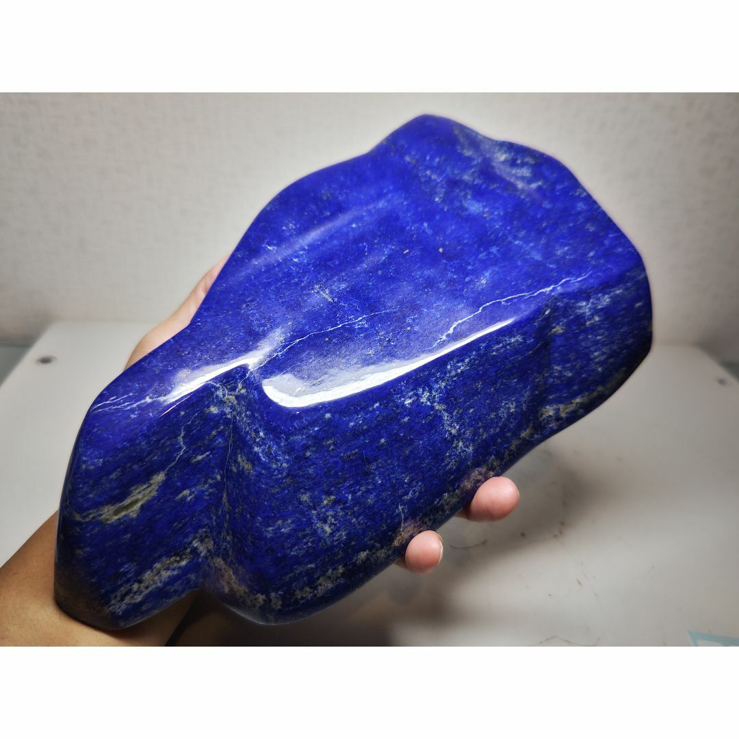
ラピスラズリ 2.8kg 原石 鑑賞石 自然石 誕生石 鉱石 鉱物 宝石 水石-


商品の情報
メルカリ安心への取り組み
お金は事務局に支払われ、評価後に振り込まれます
出品者
スピード発送
この出品者は平均24時間以内に発送しています


